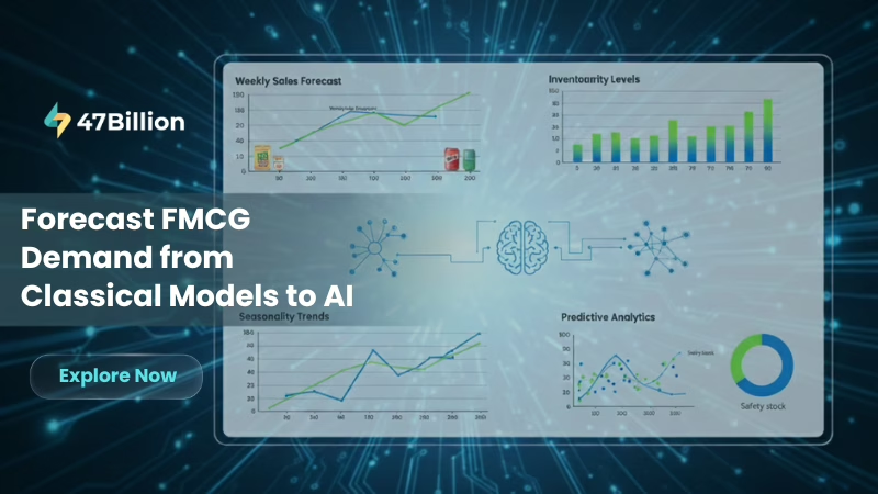
In the fast-paced world of Fast-Moving Consumer Goods (FMCG), accurate time series forecasting is essential for optimizing supply chain operations and inventory management. This guide explores FMCG demand planning strategies, transitioning from traditional statistical methods to advanced AI-driven demand forecasting techniques. Whether you’re managing SKU-level predictions in markets like India or the USA, understanding these approaches can significantly enhance supply chain efficiency.
Why Time Series Forecasting Is Critical for FMCG
FMCG companies operate in a highly volatile environment where minor forecasting inaccuracies can lead to substantial financial impacts. Over-forecasting results in surplus inventory, increased storage costs, product wastage (especially for perishable goods), and forced markdowns to clear stock. Conversely, under-forecasting causes stockouts, missed sales opportunities, eroded customer loyalty, and potential market share loss to competitors.
At its core, time series forecasting involves analyzing historical sales data to predict future demand at various levels—such as individual SKUs, stores, regions, or distribution channels. This is particularly crucial in FMCG demand planning, where products like beverages, snacks, and household essentials face rapid turnover.
FMCG organizations often grapple with challenges including:
- Short product lifecycles: New variants or seasonal items with limited historical data.
- Strong seasonality and festival effects: Spikes during holidays like Diwali in India or Black Friday in the USA.
- Promotion-driven demand spikes: Sales surges from discounts or marketing campaigns.
- Large SKU counts with limited historical data: Managing thousands of products across diverse geographies.
- Different forecasting needs across weeks, months, and quarters: Balancing short-term tactical planning with long-term strategic insights.
These issues are compounded in global markets, such as AI-driven demand planning in Europe or supply chain forecasting in the Asia-Pacific region, where economic variations and cultural events add layers of complexity. By leveraging predictive analytics in supply chain management, companies can mitigate these risks and achieve better inventory optimization for FMCG products.
This article draws from a real-world Proof-of-Concept (PoC) implemented by 47Billion’s ML team, guiding you through the evolution from classical models to machine learning and deep learning for enhanced forecasting accuracy.

Source : inciflo.com
Problem Statement: FMCG SKU-Level Forecasting
The PoC focused on a realistic scenario: forecasting weekly sales for multiple FMCG SKUs over the next 4–8 weeks, using about 104 weeks (2 years) of historical data per SKU. This setup mirrors everyday challenges in FMCG inventory optimization, such as replenishing stock in retail chains or aligning production in manufacturing.
Key constraints included:
- Weekly granularity: Capturing short-term fluctuations.
- Multiple SKUs (100+ in the dataset, PoC on 5): Scalability for high-volume portfolios.
- No external variables initially: Excluding promotions, weather, or holidays to test baseline models.
- Accuracy and explainability: Ensuring forecasts are reliable and interpretable for planners.
This approach addresses core FMCG problems in inventory planning, replenishment, and Sales & Operations Planning (S&OP) cycles, especially in geo-targeted demand planning for global markets.
Understanding Time Series Components in FMCG Data
Before diving into models, dissecting FMCG sales data is crucial. Time series data typically decomposes into four components, as outlined in various forecasting methodologies:
- Trend: The long-term direction, such as gradual market growth due to population increases or brand expansion. In FMCG, this might reflect rising demand for organic products over years.
- Seasonality: Repeating patterns at fixed intervals, like weekly peaks in weekend shopping, monthly pay-cycle boosts, or yearly surges during festivals (e.g., summer beverage sales in tropical regions like Asia-Pacific).
- Cyclicality: Irregular, longer-term fluctuations tied to economic cycles, such as recessions impacting luxury FMCG items.
- Noise (or Irregularity): Random variations from unforeseen events, like supply disruptions.
Decomposing data helps identify these elements, enabling better model selection. For instance, in FMCG trend forecasting, tools like moving averages can isolate trends from noise.

Source : fiveable.me
Stationarity: A Core Requirement for Classical Models
Many classical models assume stationarity—data with constant mean, variance, and no periodic fluctuations over time. Non-stationary data, common in FMCG due to trends and seasonality, requires transformation.
We employed the Augmented Dickey-Fuller (ADF) test to check stationarity:
- Null hypothesis: The series has a unit root (non-stationary).
- p-value < 0.05: Reject null, indicating stationarity.
- p-value ≥ 0.05: Non-stationary; apply differencing (subtracting previous values) or logarithmic transformations.
In our PoC, the FMCG SKU data was non-stationary, necessitating first-order differencing to stabilize the mean. This step is vital for models like ARIMA, as non-stationarity can lead to unreliable forecasts.
Traditional Forecasting Models (Statistical Methods)
Classical models provide interpretable baselines for time series forecasting in FMCG products.
- Exponential Smoothing (ETS):
- Captures level, trend, and seasonality using weighted averages of past observations, with recent data weighted more heavily.
- Variants include additive (constant seasonal changes) and multiplicative (proportional to level, ideal for FMCG where seasonal spikes grow with overall sales).
- In our PoC, multiplicative ETS excelled due to varying seasonal effects, such as holiday-driven proportional increases.
- ARIMA (AutoRegressive Integrated Moving Average):
- Combines autoregression (past values predict future), differencing for stationarity, and moving averages for error terms.
- Parameters: p (AR order), d (differencing), q (MA order).
- Effective for non-seasonal data but struggles with explicit seasonality; our tests showed ~30% MAPE error.
- SARIMA (Seasonal ARIMA):
- Extends ARIMA with seasonal parameters: P, D, Q, and m (seasonal period, e.g., 52 for weekly yearly cycles).
- Handles both trend and seasonality; in the PoC, with m=52, it achieved ~16.8% MAPE, the best among classics.
Conclusion (Traditional Models): For clean, seasonal FMCG data without many exogenous factors, SARIMA offers a robust, interpretable foundation, especially in regions with predictable patterns like the
Model Selection & Validation
To prevent overfitting, we used:
- AIC (Akaike Information Criterion): Balances model fit and complexity; lower is better.
- BIC (Bayesian Information Criterion): Similar but penalizes complexity more.
Evaluation metrics included:
- MAPE (Mean Absolute Percentage Error): For relative accuracy in classical models.
- MAE (Mean Absolute Error) / WAPE (Weighted Absolute Percentage Error): For ML/DL, accounting for scale.
Cross-validation via rolling forecasts ensured generalizability.
Machine Learning for FMCG Forecasting: LightGBM
LightGBM, a gradient boosting framework, excels in handling non-linear patterns and is popular in supply chain forecasting (e.g., Kaggle’s M5 competition).
Why LightGBM?
- Efficient with large datasets and categorical features.
- Leaf-wise tree growth for faster training and better accuracy on limited data.
- In FMCG, it captures subtle interactions without assuming linearity.
Feature Engineering:
- Lags: Past sales (e.g., t-1 to t-52).
- Rolling statistics: Means and std devs over windows.
- Calendar features: Week of year, holidays.
In our PoC, LightGBM outperformed LSTM due to shorter data horizons and lower computational needs, achieving superior error rates in iterative forecasting.
Deep Learning for Time Series: LSTM
Long Short-Term Memory (LSTM) networks, a type of RNN, are designed for sequential data, retaining long-term dependencies via gates (input, forget, output).
When LSTM Excels:
- Long histories and complex patterns, like multi-signal interactions in enterprise forecasting.
- Handles vanishing gradients better than vanilla RNNs.
Why It Underperformed in PoC:
- Limited ~104 weeks of data led to overfitting.
- Absence of exogenous variables reduced its edge.
- Required extensive tuning, impractical for quick PoCs.
Hybrid approaches, like ARIMA-LSTM, can boost accuracy in FMCG by combining statistical stability with neural non-linearity.
Forecast Horizon & Sliding Window Logic
For multi-week forecasts, a sliding (or rolling) window iterates predictions:
- Train on historical window, predict next step.
- Append prediction, shift window, repeat.
This supports 4–8 week horizons for advance planning, aligning manufacturing and promotions in FMCG supply chains.
Incorporating Real-World FMCG Drivers
Pure time series ignores externalities; causal forecasting integrates exogenous variables:
- Promotions & discounts: Model uplift effects.
- Festivals & holidays: Account for spikes (e.g., Christmas in Europe).
- Weather: Impacts seasonal goods like ice cream.
- Regional events, price changes, channel shifts: Geo-specific factors.
Adding these via models like SARIMAX or ML reduces errors by 20-30% in practice.
Traditional vs ML vs Deep Learning: How to Decide?
| Scenario | Best Approach | Rationale |
| Clear seasonality, small data | SARIMA / ETS | Simple, interpretable; suits limited histories. |
| Medium complexity, limited data | LightGBM | Handles non-linearity efficiently. |
| Long history, complex patterns | LSTM / Transformers | Captures deep dependencies. |
| Multi-signal enterprise forecasting | Hybrid / Ensemble (e.g., TFT) | Combines strengths for interpretable multi-horizon predictions. |
Emerging models like Temporal Fusion Transformers (TFT) integrate attention mechanisms with LSTM-like encoders for enhanced interpretability and handling of static/dynamic covariates in large-scale FMCG enterprises.
How 47Billion Helps FMCG Organizations
As a premier AI-driven product engineering and software development company, 47Billion specializes in embedding machine learning into supply chain solutions. We don’t just deploy models—we architect end-to-end systems tailored to FMCG needs, leveraging data analytics for smarter decisions.
Our offerings include:
- SKU/Store/Region-level forecasting: Customized for geo-targeted markets like India or the USA.
- Traditional + ML + DL ensemble pipelines: Blending ARIMA with LightGBM/LSTM for hybrid accuracy.
- Promotion & event-aware forecasting: Incorporating exogenous variables for real-time adjustments.
- Accuracy monitoring & drift detection: Ensuring models adapt to changing patterns.
- UI dashboards for planners: Intuitive interfaces for demand sensing.
- Integration with ERP/SCM systems: Seamless connectivity for operational efficiency.
By partnering with 47Billion, FMCG teams transition from manual spreadsheets to AI-assisted demand intelligence, driving efficiency and growth. Learn more at https://47billion.com/.

Final Takeaways
- Time series forecasting in FMCG is highly context-dependent, varying by region and product.
- Classical models like SARIMA remain relevant for baselines.
- ML approaches like LightGBM excel with feature engineering.
- Deep learning, including LSTM and TFT, thrives on scale and rich data.
- True value emerges from integrated platforms, as provided by solution experts like 47Billion, transforming data into actionable insights for global supply chains.